TensorFlow. Create, Train, and Use a Simple Model
In the world of machine learning and artificial intelligence, TensorFlow stands out due to its flexibility and powerful capabilities. In this article, I'll show the process of creating a simple TensorFlow model to demonstrate how easy it is to get started with this tool.
Whether you are new to machine learning or an experienced developer, this step-by-step guide will help you understand the basic concepts and methods behind building models using TensorFlow.
Linear Regression
To understand the basic mechanism behind TensorFlow, I use Celsius to Fahrenheit conversion formula:
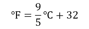
It's a simple linear function that describes the relationship between two variables: the Celsius (°C) and Fahrenheit (°F) temperatures. The dependent variable in this equation is the Fahrenheit temperature, and the independent variable is the Celsius temperature. The constants in the equation are the gradient (9/5) and the intercept (32). Other constants in the formula include "gradient" (9/5) and "intercept" (32).
With TensorFlow, we can create a model that predicts the dependent variable based on the independent one.
Objectives
The goal is to create and train a TensorFlow model that can predict the Celsius to Fahrenheit conversion, without knowing the exact formula. The model needs to learn the gradient and intercept values from a small dataset, using a large number of training iterations.
Prerequisites
To work with TensorFlow models, you will need two libraries open-source Python libraries:
NumPy (Numerical Python). It provides support for large, multi-dimensional arrays and matrices, along with a collection of mathematical functions to operate on these arrays efficiently. TensorFlow developed by Google, is a powerful tool for machine learning and artificial intelligence applications.
Note
This article based on TensorFlow version 2.17.0 and NumPy version 1.26.4.
To install the libraries with the pip run the following commands in terminal:
pip install tensorflow
pip install numpy
For more information on how to install TensorFlow, please refer to the official guide: Install TensorFlow 2.
Dataset
To train the model, we need a dataset that provides input data and corresponding output. For this purpose, let's use the values from 0 to 15 in Celsius and their corresponding values in Fahrenheit.
| Celsius | Fahrenheit |
|---|---|
| 0 | 32 |
| 1 | 33.8 |
| 2 | 35.6 |
| 3 | 37.4 |
| 4 | 39.2 |
| 5 | 41 |
| 6 | 42.8 |
| 7 | 44.6 |
| 8 | 46.4 |
| 9 | 48.2 |
| 10 | 50 |
| 11 | 51.8 |
| 12 | 53.6 |
| 13 | 55.4 |
| 14 | 57.2 |
| 15 | 59 |
Let's create two lists, one for the Celsius values and one for the Fahrenheit values. We will fill these lists with the calculated values of the temperature conversion.
# Independent variables
temp_c = []

# Dependent variables
temp_f = []

# Fill the arrays with calculated values
for c in range(0, 16):
    f = 32 + 1.8 * c
    temp_c.append(float(c))
    temp_f.append(float(f))

# Input array
input_array = np.array(temp_c, dtype=float)

# Correct values for the input array
output_array = np.array(temp_f, dtype=float)
We'll use these two lists to train our model.
Model
The following code creates a new sequential model:
model = tf.keras.Sequential()
First, we need to define the input for the model. In this case, it's going to be a one-dimensional array (shape=[1]):
model.add(tf.keras.layers.Input(shape=[1]))
Next, we create a densely connected neural network layer using the tf.keras.layers.Dense function, with a single output dimension (units=1).
model.add(tf.keras.layers.Dense(units=1))
The Dense layer provides a bias vector and a kernel weights matrix. The bias is used to predict the "intercept", and the kernel is used for the "gradient".
The model takes a single-dimensional array (temperature in Celsius) as input and produces a single-dimensional array (temperature in Fahrenheit) as output.
Once the model has been defined, we can compile it and specify the training configuration, including the optimizer, loss function, and optional metrics. I use the built-in optimizer (SGD) and mean squared error loss function (MeanSquaredError).
model.compile(optimizer=tf.keras.optimizers.SGD(), loss=tf.keras.losses.MeanSquaredError())
We can also choose to include additional metrics, if desired. Other loss functions and optimizers can be used, or you can create your own custom ones.
Before training the model, let's take a look at the weights of the Dense layer by calling the get_wieghts method of the layer:
model.layers[0].get_weights()
In my case, the gradient is -0.81139004 and the intercept is 0. These are random values that may change during the training process, depending on the loss and optimizer used.
Note
The model can be used for prediction without any training, as the weights have already been set.
Train the Model
Now, we can train the model by specifying the number of iterations. An iteration is an entire cycle through the input and output data.
model.fit(input_array, output_array, epochs=100)
Weights
We know that the gradient is 9/5 and the intercept is 32. However, the model still needs to predict values. In the images below, you can see how the weights of the model have changed during the training process.
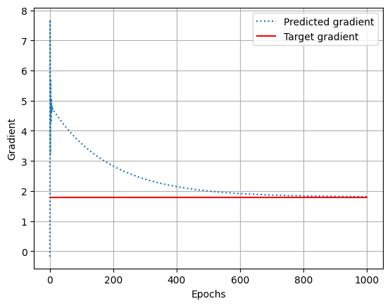
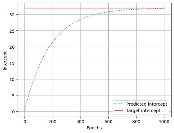
After 1000 epochs of training, the gradient is 1.8131773 and the intercept is 31.864311. These values are quite close to the real values we know (1.8 and 32), which is good.
Note
The process of training the model is to select the weights in accordance with loss and optimizer.
Using the Model
To use the model to predict values, we need to call the predict method and provide the input:
# Temperature in Celsius
temp_c = [0,1,2,3,4,5]

# Predicted temperature in Fahrenheit
temp_f = model.predict(np.array(temp_c))

print(temp_f)
Ouput:
[[31.864311]
 [33.67749 ]
 [35.490665]
 [37.303844]
 [39.11702 ]
 [40.9302  ]]
Model Accuracy
The following graph shows the results of converting the temperature values from Celsius to Fahrenheit using the same model, but with a different numbers of training iterations (epochs):
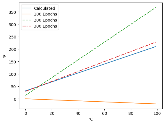
After 100 training iterations, the model's predictions are not very accurate (orange line). However, after 300 iterations, the quality of the predictions improves.
Save/Load Model
You can save the entire model, including the architecture, weights, and optimizer state, by using the save method:
model.save("c_to_f_conversion.h5")
To load the saved model use the load_weights method:
from tensorflow.keras.models import load_model

model = load_model("c_to_f_conversion.h5")
Summary
I hope this article will be helpful for beginners who want to gain practical experience with TensorFlow and learn the basics of creating and training machine learning models.
GitHub
Jupyter Notebook is available on my github repo: https://github.com/vzhukov/tensorflow-samples.